Tutorial
This tutorial shows the basic steps of using SEP to detect objects in an image and perform some basic aperture photometry.
Here, we use the fitsio package, just to read the test image, but
you can also use astropy.io.fits for this purpose (or any other FITS
reader).
In [1]:
import numpy as np
import sep
In [2]:
# additional setup for reading the test image and displaying plots
import fitsio
import matplotlib.pyplot as plt
from matplotlib import rcParams

%matplotlib inline

rcParams['figure.figsize'] = [10., 8.]
/usr/lib/python3/dist-packages/matplotlib/font_manager.py:273: UserWarning: Matplotlib is building the font cache using fc-list. This may take a moment.
  warnings.warn('Matplotlib is building the font cache using fc-list. This may take a moment.')
/usr/lib/python3/dist-packages/matplotlib/font_manager.py:273: UserWarning: Matplotlib is building the font cache using fc-list. This may take a moment.
  warnings.warn('Matplotlib is building the font cache using fc-list. This may take a moment.')
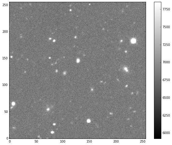
First, we’ll read an example image from a FITS file and display it, just to show what we’re dealing with. The example image is just 256 x 256 pixels.
In [3]:
# read image into standard 2-d numpy array
data = fitsio.read("../data/image.fits")
In [4]:
# show the image
m, s = np.mean(data), np.std(data)
plt.imshow(data, interpolation='nearest', cmap='gray', vmin=m-s, vmax=m+s, origin='lower')
plt.colorbar();
Background subtraction
Most optical/IR data must be background subtracted before sources can be detected. In SEP, background estimation and source detection are two separate steps.
In [5]:
# measure a spatially varying background on the image
bkg = sep.Background(data)
There are various options for controlling the box size used in estimating the background. It is also possible to mask pixels. For example:
bkg = sep.Background(data, mask=mask, bw=64, bh=64, fw=3, fh=3)
See the reference section for descriptions of these parameters.
This returns an Background object that holds information on the
spatially varying background and spatially varying background noise
level. We can now do various things with this Background object:
In [6]:
# get a "global" mean and noise of the image background:
print(bkg.globalback)
print(bkg.globalrms)
6852.04931640625
65.46165466308594
In [7]:
# evaluate background as 2-d array, same size as original image
bkg_image = bkg.back()
# bkg_image = np.array(bkg) # equivalent to above
In [8]:
# show the background
plt.imshow(bkg_image, interpolation='nearest', cmap='gray', origin='lower')
plt.colorbar();

In [9]:
# evaluate the background noise as 2-d array, same size as original image
bkg_rms = bkg.rms()
In [10]:
# show the background noise
plt.imshow(bkg_rms, interpolation='nearest', cmap='gray', origin='lower')
plt.colorbar();

In [11]:
# subtract the background
data_sub = data - bkg
One can also subtract the background from the data array in-place by
doing bkg.subfrom(data).
Warning:
If the data array is not background-subtracted or the threshold is too
low, you will tend to get one giant object when you run object detection
using sep.extract. Or, more likely, an exception will be raised due
to exceeding the internal memory constraints of the sep.extract
function.
Object detection
Now that we’ve subtracted the background, we can run object detection on the background-subtracted data. You can see the background noise level is pretty flat. So here we’re setting the detection threshold to be a constant value of \(1.5 \sigma\) where \(\sigma\) is the global background RMS.
In [12]:
objects = sep.extract(data_sub, 1.5, err=bkg.globalrms)
sep.extract has many options for controlling detection threshold,
pixel masking, filtering, and object deblending. See the reference
documentation for details.
objects is a NumPy structured array with many fields.
In [13]:
# how many objects were detected
len(objects)
Out[13]:
68
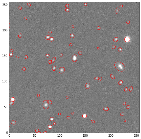
objects['x'] and objects['y'] will give the centroid coordinates
of the objects. Just to check where the detected objects are, we’ll
over-plot the object coordinates with some basic shape parameters on the
image:
In [14]:
from matplotlib.patches import Ellipse

# plot background-subtracted image
fig, ax = plt.subplots()
m, s = np.mean(data_sub), np.std(data_sub)
im = ax.imshow(data_sub, interpolation='nearest', cmap='gray',
               vmin=m-s, vmax=m+s, origin='lower')

# plot an ellipse for each object
for i in range(len(objects)):
    e = Ellipse(xy=(objects['x'][i], objects['y'][i]),
                width=6*objects['a'][i],
                height=6*objects['b'][i],
                angle=objects['theta'][i] * 180. / np.pi)
    e.set_facecolor('none')
    e.set_edgecolor('red')
    ax.add_artist(e)
objects has many other fields, giving information such as second
moments, and peak pixel positions and values. See the reference
documentation for sep.extract for descriptions of these fields. You
can see the available fields:
In [15]:
# available fields
objects.dtype.names
Out[15]:
('thresh',
 'npix',
 'tnpix',
 'xmin',
 'xmax',
 'ymin',
 'ymax',
 'x',
 'y',
 'x2',
 'y2',
 'xy',
 'errx2',
 'erry2',
 'errxy',
 'a',
 'b',
 'theta',
 'cxx',
 'cyy',
 'cxy',
 'cflux',
 'flux',
 'cpeak',
 'peak',
 'xcpeak',
 'ycpeak',
 'xpeak',
 'ypeak',
 'flag')
Aperture photometry
Finally, we’ll perform simple circular aperture photometry with a 3 pixel radius at the locations of the objects:
In [16]:
flux, fluxerr, flag = sep.sum_circle(data_sub, objects['x'], objects['y'],
                                     3.0, err=bkg.globalrms, gain=1.0)
flux, fluxerr and flag are all 1-d arrays with one entry per
object.
In [17]:
# show the first 10 objects results:
for i in range(10):
    print("object {:d}: flux = {:f} +/- {:f}".format(i, flux[i], fluxerr[i]))
object 0: flux = 2249.173164 +/- 291.027422
object 1: flux = 3092.230000 +/- 291.591821
object 2: flux = 5949.882168 +/- 356.561539
object 3: flux = 1851.435000 +/- 295.028419
object 4: flux = 72736.400605 +/- 440.171830
object 5: flux = 3860.762324 +/- 352.162684
object 6: flux = 6418.924336 +/- 357.458504
object 7: flux = 2210.745605 +/- 350.790787
object 8: flux = 2741.598848 +/- 352.277244
object 9: flux = 20916.877324 +/- 376.965683
Finally a brief word on byte order
Note:
If you are using SEP to analyze data read from FITS files with astropy.io.fits you may see an error message such as:
ValueError: Input array with dtype '>f4' has non-native byte order.
Only native byte order arrays are supported. To change the byte
order of the array 'data', do 'data = data.byteswap().newbyteorder()'
It is usually easiest to do this byte-swap operation directly after reading the array from the FITS file. You can even perform the byte swap in-place by doing
>>> data = data.byteswap(inplace=True).newbyteorder()
If you do this in-place operation, ensure that there are no other
references to data, as they will be rendered nonsensical.
For the interested reader, this byteswap operation is necessary because astropy.io.fits always returns big-endian byte order arrays, even on little-endian machines. For more on this, see