Matched Filter (Convolution)

For source detection, SEP supports using a matched filter, which can give the optimal detection signal-to-noise for objects with some known shape. This is controlled using the filter_kernel keyword in sep.extract. For example:

kernel = np.array([[1., 2., 3., 2., 1.],
                   [2., 3., 5., 3., 2.],
                   [3., 5., 8., 5., 3.],
                   [2., 3., 5., 3., 2.],
                   [1., 2., 3., 2., 1.]])
objects = sep.extract(data, thresh, filter_kernel=kernel)

If filter_kernel is not specified, a default 3-by-3 kernel is used. To disable filtering entirely, specify filter_kernel=None.

What array should be used for filter_kernel? It should be approximately the shape of the objects you are trying to detect. For example, to optimize for the detection of point sources, filter_kernel should be set to shape of the point spread function (PSF) in the data. For galaxy detection, a larger kernel could be used. In practice, anything that is roughly the shape of the desired object works well since the main goal is to negate the effects of background noise, and a reasonable estimate is good enough.

Correct treatment in the presence of variable noise

In Source Extractor, the matched filter is implemented assuming there is equal noise across all pixels in the kernel. The matched filter then simplifies to a convolution of the data with the kernel. In sep.extract, this is also the behavior when there is constant noise (when err is not specified).

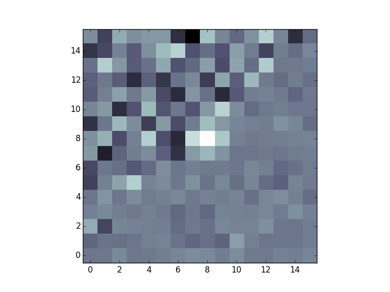
In the presence of independent noise on each pixel, SEP uses a full matched filter implementation that correctly accounts for the noise in each pixel. This is not available in Source Extractor. Some benefits of this method are that detector sensitivity can be taken into account and edge effects are handled gracefully. For example, suppose we have an image with noise that is higher in one region than another. This can often occur when coadding images:

# create a small image with higher noise in the upper left
n = 16
X, Y = np.meshgrid(np.arange(n), np.arange(n))
mask = Y > X
error = np.ones((n, n))
error[mask] = 4.0
data = error * np.random.normal(size=(n, n))

# add source to middle of data
source = 3.0 * np.array([[1., 2., 1.],
                         [2., 4., 2.],
                         [1., 2., 1.]])
m = n // 2 - 1
data[m:m+3, m:m+3] += source

plt.imshow(data, interpolation='nearest', origin='lower', cmap='bone')

Specifying filter_type='conv' will use simple convolution, matching the behavior of Source Extractor. The object is not detected:

>>> objects = sep.extract(data, 3.0, err=error, filter_type='conv')
>>> len(objects)
0

Setting filter_type='matched' (the default) correctly deweights the noisier pixels around the source and detects the object:

>>> objects = sep.extract(data, 3.0, err=error, filter_type='matched')
>>> len(objects)
1

Derivation of the matched filter formula

Assume that we have an image containing a single point source. This produces a signal with PSF \(S_i\) and noise \(N_i\) at each pixel indexed by \(i\). Then the measured image data \(D_i\) (i.e. our pixel values) is given by:

\[D_i = S_i + N_i\]

Then we want to apply a linear transformation \(T_i\) which gives an output \(Y\):

\[Y = \sum_i T_i D_i = T^T D\]

We use matrix notation from here on and drop the explicit sums. Our objective is to find the transformation \(T_i\) which maximizes the signal-to-noise ratio \(SNR\).

\[SNR^2 = \frac{(T^T S)^2}{E[(T^T N)^2]}\]

We can expand the denominator as:

\[E[(T^T N)^2] = E[(T^T N)(N^T T)] = T^T \cdot E[N N^T] \cdot T = T^T C T\]

Where \(C_{ik}\) is the covariance of the noise between pixels \(i\) and \(k\). Now using the Cauchy-Schwarz inequality on the numerator:

\[(T^T S)^2 = (T^T C^{1/2} C^{-1/2} S)^2 \le (T^T C^{1/2})^2 (C^{-1/2} S)^2 = (T^T C T) (S^T C^{-1} S)\]

since \(C^T = C\). The signal-to-noise ratio is therefore bounded by:

\[\begin{split}&SNR^2 \le \frac{(T^T C T)(S^T C^{-1} S)}{(T^T C T)} \\ &SNR^2 \le S^T C^{-1} S\end{split}\]

Choosing \(T = \alpha C^{-1} S\) where \(\alpha\) is an arbitrary normalization constant, we get equality. Hence this choise of \(T\) is the optimal linear tranformation. We normalize this linear transformation so that if there is no signal and only noise, we get an expected signal-to-noise ratio of 1. With this definition, the output \(SNR\) represents the number of standard deviations above the background. This gives:

\[\begin{split}&E[(T^T N)^2] = T^T C T = \alpha^2 S^T C^{-1} C C^{-1} S = \alpha^2 S^T C^{-1} S = 1 \\ &\alpha = \frac{1}{\sqrt{S^T C^{-1} S}}\end{split}\]

Putting everything together, our normalized linear transformation is:

\[T = \frac{C^{-1} S}{\sqrt{S^T C^{-1} S}}\]

And the optimal signal-to-noise is given in terms of the known variables as:

\[SNR = \frac{S^T C^{-1} D}{\sqrt{S^T C^{-1} S}}\]